Multi-stage interpolation.

Design a two-stage interpolation with a total interpolation factor of four.

import math

import matplotlib.pyplot as plt
import numpy as np
from mplsignal import freqz_fir

from fird.constraint import PiecewiseLinearConstraint
from fird.designer import FIRDesigner
from fird.objective import PiecewiseLinearObjective
from fird.util import expand

Obtimize stopband attentation, while keeping passband ripple below 0.01

total_objective = PiecewiseLinearObjective([0.3, 0.7, 0.8, 1], [0, 0, 0, 0])
total_constraint = PiecewiseLinearConstraint([0, 0.2], [1, 1], [0.01])

Design first stage filter, keep passband ripple to half

firststage_objective = PiecewiseLinearObjective([0.6, 1], [0, 0])
firststage_constraint = PiecewiseLinearConstraint([0, 0.4], [1, 1], [0.01 / 2])
firststage_designer = FIRDesigner(31, firststage_objective, firststage_constraint)
firststage_designer.solve()
h1 = firststage_designer.get_impulse_response()

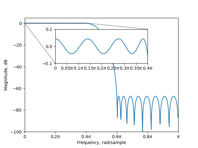
Plot the magnitude response of the first-stage filter.

fig, ax = plt.subplots()
freqz_fir(h1, ax=ax, style="magnitude")
axins = ax.inset_axes(
    [0.2, 0.6, 0.6, 0.3],
)
ax.set_ylim((-100, 5))
freqz_fir(h1, ax=axins, style="magnitude")
axins.set_xlim(0, 0.4 * np.pi)
axins.set_ylim(-0.1, 0.1)
axins.xaxis.label.set_visible(False)
axins.yaxis.label.set_visible(False)
ax.indicate_inset_zoom(axins, edgecolor="black")
fig.show()

Design second-stage filter subject to an upsampled version of the first-stage filter. From now on, the total objective and constraint is used.

upsampled_h1 = expand(h1, 2)
secondstage_designer = FIRDesigner(
    17, total_objective, total_constraint, cascade_filter=upsampled_h1
)
secondstage_designer.solve()
h2 = secondstage_designer.get_impulse_response()
print(
    f"Minimum stopband attenuation: {-20 * math.log10(secondstage_designer.objective_value)} dB"
)

Minimum stopband attenuation: 72.4954747000503 dB

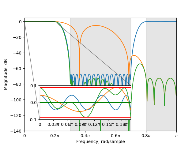
Plot the different filters and the total response

combined = np.convolve(upsampled_h1, h2)
fig, ax = plt.subplots()
freqz_fir(upsampled_h1, ax=ax, style="magnitude")
freqz_fir(h2, ax=ax, style="magnitude")
freqz_fir(combined, ax=ax, style="magnitude")
total_objective.plot(ax=ax, plot_db=True, plot_range=True)
ax.set_ylim((-140, 5))
axins = ax.inset_axes([0.1, 0.1, 0.6, 0.3])
freqz_fir(upsampled_h1, ax=axins, style="magnitude")
freqz_fir(h2, ax=axins, style="magnitude")
freqz_fir(combined, ax=axins, style="magnitude")
total_constraint.plot(ax=axins, plot_db=True)
axins.set_xlim(0, 0.2 * math.pi)
axins.set_ylim(-0.1, 0.1)
axins.xaxis.label.set_visible(False)
axins.yaxis.label.set_visible(False)
ax.indicate_inset_zoom(axins, edgecolor="black")
fig.show()

/builds/oscgu95/fird/venv/lib/python3.13/site-packages/fird/util.py:58: RuntimeWarning: divide by zero encountered in log10
  return -20 * np.log10(np.abs(a))

Now redesign the first-stage filter subject to the second-stage filter. As the first-stage filter is periodic when considering the the final sample rate, the period argument is used.

firststage_redesigner = FIRDesigner(
    31, total_objective, total_constraint, cascade_filter=h2, period=2
)
firststage_redesigner.solve()
h1_new = firststage_redesigner.get_impulse_response()
print(
    f"Minimum stopband attenuation: {-20 * math.log10(firststage_redesigner.objective_value)} dB"
)

Minimum stopband attenuation: 72.49532277396742 dB

Plot the new and old first-stage filters.

fig, ax = plt.subplots()
freqz_fir(h1_new, ax=ax, style="magnitude")
freqz_fir(h1, ax=ax, style="magnitude")
ax.set_ylim((-100, 5))
axins = ax.inset_axes([0.2, 0.6, 0.6, 0.3])
freqz_fir(h1_new, ax=axins, style="magnitude")
freqz_fir(h1, ax=axins, style="magnitude")
axins.set_xlim(0, 0.4 * math.pi)
axins.set_ylim(-0.1, 0.1)
axins.xaxis.label.set_visible(False)
axins.yaxis.label.set_visible(False)
ax.indicate_inset_zoom(axins, edgecolor="black")
fig.show()

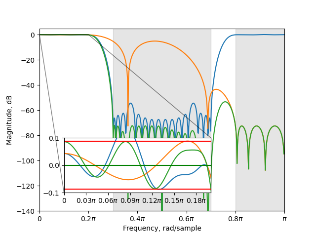
The new first-stage filter does not lead to an improved total response.

upsampled_h1_new = expand(h1_new, 2)
combined_new = np.convolve(upsampled_h1_new, h2)

fig, ax = plt.subplots()
freqz_fir(upsampled_h1_new, ax=ax, style="magnitude")
freqz_fir(h2, ax=ax, style="magnitude")
freqz_fir(combined_new, ax=ax, style="magnitude")
total_objective.plot(ax=ax, plot_db=True, plot_range=True)
ax.set_ylim((-140, 5))
axins = ax.inset_axes([0.1, 0.1, 0.6, 0.3])
freqz_fir(upsampled_h1_new, ax=axins, style="magnitude")
freqz_fir(h2, ax=axins, style="magnitude")
freqz_fir(combined_new, ax=axins, style="magnitude")
total_constraint.plot(ax=axins, plot_db=True)
axins.set_xlim(0, 0.2 * np.pi)
axins.set_ylim(-0.1, 0.1)
axins.xaxis.label.set_visible(False)
axins.yaxis.label.set_visible(False)
ax.indicate_inset_zoom(axins, edgecolor="black")
fig.show()

Redesign second-stage filter subject to an upsampled version of the redesigned first-stage filter.

secondstage_redesigner = FIRDesigner(
    17, total_objective, total_constraint, cascade_filter=upsampled_h1_new
)
secondstage_redesigner.solve()
h2_new = secondstage_redesigner.get_impulse_response()
print(
    f"Minimum stopband attenuation: {-20 * math.log10(secondstage_redesigner.objective_value)} dB"
)

Minimum stopband attenuation: 73.25777146258964 dB

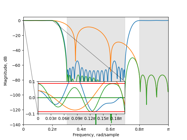
Plot the different filters and the total response.

combined = np.convolve(upsampled_h1_new, h2_new)
fig, ax = plt.subplots()
freqz_fir(upsampled_h1_new, ax=ax, style="magnitude")
freqz_fir(h2_new, ax=ax, style="magnitude")
freqz_fir(combined, ax=ax, style="magnitude")
total_objective.plot(ax=ax, plot_db=True, plot_range=True)
ax.set_ylim((-140, 5))
axins = ax.inset_axes([0.1, 0.1, 0.6, 0.3])
freqz_fir(upsampled_h1_new, ax=axins, style="magnitude")
freqz_fir(h2_new, ax=axins, style="magnitude")
freqz_fir(combined, ax=axins, style="magnitude")
total_constraint.plot(ax=axins, plot_db=True)
axins.set_xlim(0, 0.2 * math.pi)
axins.set_ylim(-0.1, 0.1)
axins.xaxis.label.set_visible(False)
axins.yaxis.label.set_visible(False)
ax.indicate_inset_zoom(axins, edgecolor="black")
fig.show()

It may now be possible to obtain a slightly better second-stage filter and so on. However, as the combined filter is a non-convex problem, it may not converge to the global minimum.